Data
Allele specific binding (ASB) data for various transcription factors were retrieved from the ADASTRA database (Abramov et al. 2021) and a eY1H experiment (Bass et al. 2015). Training was conducted on chip-seq data from ADASTRA source experiments. SNPeBoT in its current iteration makes its prediction solely on the effect of Nucleotides 7 basepairs up and downstream of the mutation (or the midpoint of a 51bp sequence as the case would be for insertions, deletions or multiple mutations), therefore all ADASTRA derived non-concordant ASB events were discarded to controll for off-site effects on ASB. After this filtration step 34374 data points remained for 219 Different Transcription Factors (TFs).
Further filtering out of data was conducted for datapoints where the relevant TF could not be assigned to a PBM motif, and all duplicate ASBs were removed. This resulted in 9215 ASBs for which Transcription Factors experienced either a gain or loss in binding. To add no change data (control SNPs) we took a further 8996 SNPs from the ADASTRA source experiments that had no significant ASB measured and added these to the total training set which was composed of 18211 data points.
The eY1H data, in full, was reserved for testing. After data processing, as conducted on the ADASTRA set, we retained a total of 52 ASB events from an initial set of 294. Unlike chip-seq experiments, which may be influenced by the context in which SNPs occur, any effect measured in eY1H experiments will be down to changes in a TFs affinity to the nucleotide sequence at the binding site.
Data Processing
A single SNP prediction has to undergo multiple levels of processing to yield the input features upon which the prediction is made. First the amino acid sequence of the TF acting upon the SNP is retrieved and compared against a database of motifs, for which PBM experiments have been performed, using BLAST (Altschul et al. 1990). Any motif with 70% or more sequence identity with the query TF is selected as a match. This preprocessing step was handled by SBILib (Gohl et al. 2023). Reference and Alternate sequences are retrieved from the UCSC genome browser (Raney et al. 2024) or genopyc (Gualdi et al. 2024) for VCF or RSID input format respectively.
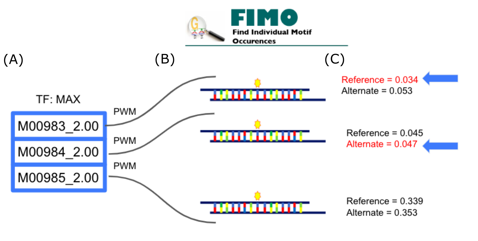
Subsequently the PWMs for these motifs are scanned against both the alternate and reference sequences using FIMO (Grant et al. 2011). For each sequence the motif with the best scoring FIMO hit incorporating the mutated position is selected as the binding motif Fig 1. The best binding hits from FIMO with these motifs is saved for later use in training. For each sequence the relevant motif associated E-scores for all octomers incorporating the mutated position are retrieved, for a total of 16. Next a sliding window of average E-scores is assigned to each Nucleotide part of these octomers, 7 bases up and downstream of the mutated position, yielding a total of 30 E-score averages (15 for the reference and alternate sequences respectively), in addition to the 2 p-values stemming from the best FIMO hits. These 32 scores were then transformed into a 8x4 matrix.
Model
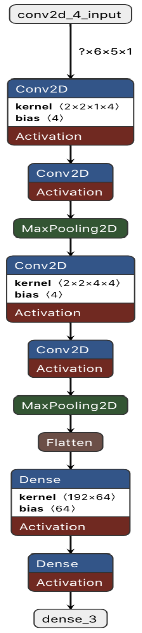
We trained a Convolutional Neural Network (Fig. 2) using Tensorflow (Abadi et al. 2016). The model takes an input (8,4,1) feature matrix. This is passed on two two initial 2D convolution layers and a pooling layer, followed by a second set of 2 convolution and 1 pooling layer. After normalizaton the data is flattened and passed to 2 Dense layers with a final softmax activation function giving the model a 3 class output corresponding to the probability summing to 1 of each prediction “gain”, “loss”,”no-change” in binding. To train the model our dataset was split into 70% of the smallest class (gain) and matching these with the remaining 2 classes so that the training set (8877 ASBs) was balanced, all remaining point went to a hold-out test set (8400 ASBs). From the training set a further split was made yielding a 10% validation set (934 ASBs). All data was shuffled prior to the splits to ensure proper class representation.
Post-Hoc Control
Holdout testing of the CNN model prior to inclusion of the post-Hoc filter achieved 81% accuracy at 62% ASB recall with no distinction applied between the TFs for which predictions were made. When predictions were run on unseen SNPs regardless of the TF, the model achieved an accuracy of 80% with a 61% ASB recall rate. Accuracy and ASB recall when predicting on TFs not included in training for any SNPs was 83%. In order to account for cases where ASB was not solely due to alteration in DNA sequence at the binding site we implemented a Post-Hoc control method to ensure that there is an effect of the SNP on TF binding Fig 3.

Supplementary generalizability Test
When testing on AlleleDB (Chen et al. 2016) ASB events, preprocessing of data for PBM-included TFs significantly reduced the number of ASBs as the database was extremely biased to a small number of TFs with 5 Non-SNPeBoT applicable TFs making up 92% of the data. The testable ASB number was further restricted by other TFs not available for SNPeBoT to test on. On this small dataset SNPeBoT received an accuracy and ASB recall rate of 19%, however it also attained a True Positive Rate of 76%. This highlights the main weakness of SNPeBoT in its reliance on the availability of PBM data, however as more PBM data becomes available and is included in SNPeBoT this will be ameliorated. Crucially, even at this level the True Positive rate remains high with accuracy lower than on the AdAstra Test set due to the fact that SNPeBoT overpredicted no-change in a data set containing only gain or loss classifications.
Benchmarking
The post-hoc included predictions of SNPeBoT on test data were compared with predictions of two established tools for prediction ASB, MotifbreakR (Coetzee et al. 2015) and atSNP (Zuo et al. 2015). Both tools are available as R packages and were installed with all necessary dependencies. For both MotifbreakR and atSNP we followed the provided vignette tutorials. In MotifbreakR each transcription factor had its motifs queried from MotifDB and predictions on SNPs were made for these motifs scoring with the relative entropy method at a threshold of 1e-4. Because MotifbreakR doesn’t select a motif to apply to each SNP we frequently retrieved multiple predictions per SNP, corresponding to the various motifs for the given TF. To resolve this we looked at the average allele difference for each prediction per SNP. Classification were based on these averages, either “loss” or “gain”. When predicted values were 0 or the no predictions were returned the SNP was classified as “no-change”.
For atSNP each TFs publicly available PWMs from the CISBP database (Weirauch et al. 2014) were downloaded. Affinity scores and p-values and applied multiple testing adjustment using Storey’s q-value with the qvalue package (Storey et al. 2023) were calculated. We applied a qval_rank <= 0.05 filter to retrieve effect predictions. As with motifbreakR this left us with multiple predictions per SNP, reflecting the number of PWMs per TF, for which we employed the same method to retrieve a single prediction. Prediction accuracy and Allele Specific Binding recall rate were calculated for both MotifbreakR, atSNP and SNPeBoT. The results for each tool from 9 diffferent thresholds were then compared.
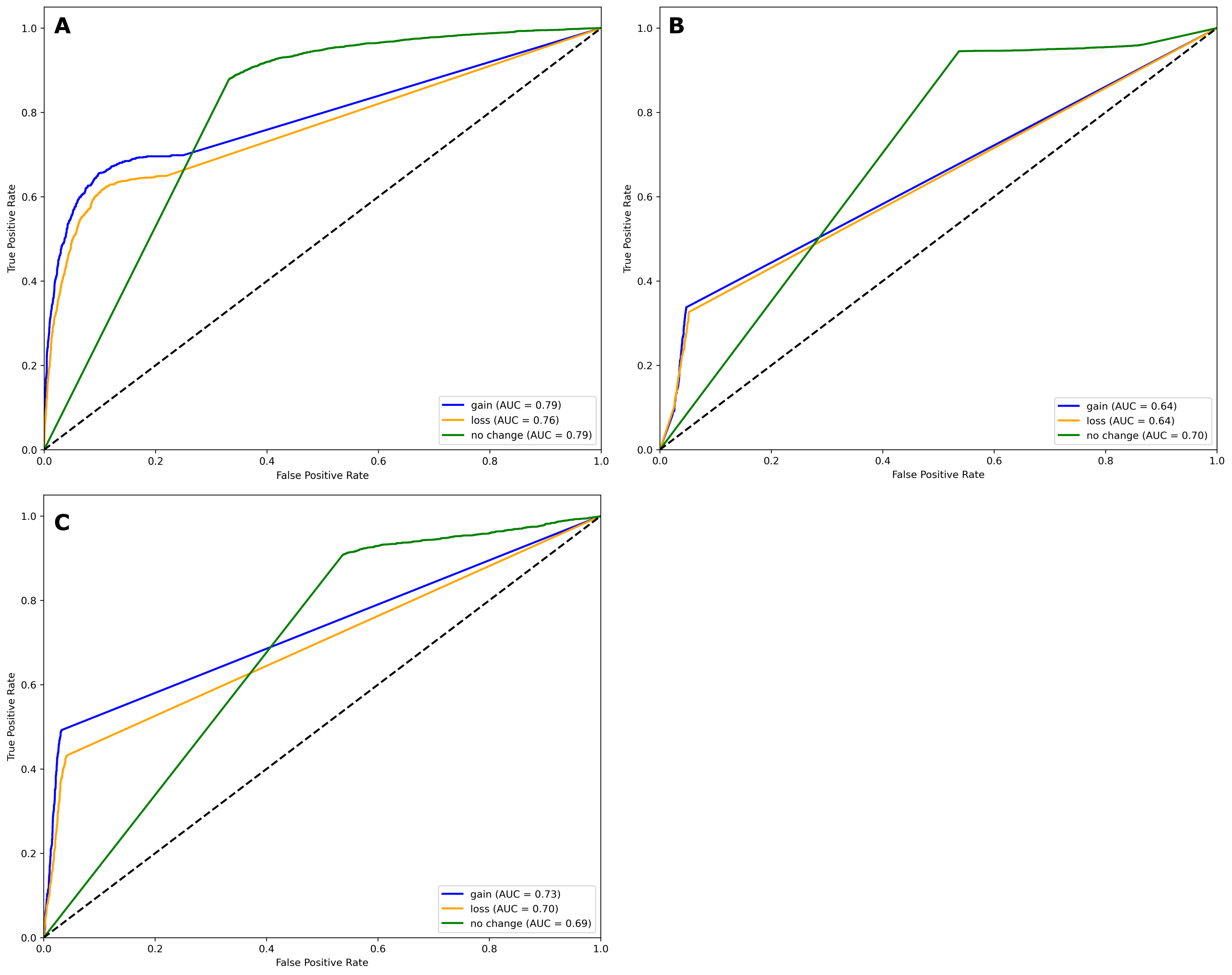
Next the area under the receiver operating characteristic curve was calculated for all three classes of predictions at their best performing threshold (based on accuracy of predictions). Due to the nature of ROC curve generation we were limited to classes that received a probability measure, since no-change classifications for atSNP and motifbreakR were any cases that did not return significant predictions. To generate class probability measures for motifbreakR we took the absolute value of the returned prediction (ranging from -2 to 2) and normalized it to a range between 0 and 1. This represented the probability of the predicted class, the non-predicted class was assigned the complementary probability. For atSNP we first computed the p-value difference in reference and alternate allele in a log transformed space. Probabilities were then assigned to the predicted class based on a sigmoid scaling of the difference with the alternate class receiving the complementary probability.
Results
Holdout testing of the CNN model prior to inclusion of the post-Hoc filter achieved 81% accuracy at 62% ASB recall with no distinction applied between the TFs for which predictions were made. When predictions were run on unseen SNPs regardless of the TF, the model achieved an accuracy of 80% with a 61% ASB recall rate. Accuracy and ASB recall when predicting on TFs not included in training for any SNPs was 83%. Results for Benchmarking Tests can be seen in Fig 4. SNPeBoT produces greater accuracy than a PWM only approach and both Benchmarking tools tested. SNPeBoT was also able to find more Allele Specific Binding SNPs than the other tested tools.



Usage
Any submission must follow one of the three formats: VCF, Sequence, or rsid. We have provided examples and explanation to each fomat type on the Home page. For the webserver there are specific limits of SNPs that may be submitted for each Format type in the single TF prediction mode (Sequence:30, VCF:15, RSID: 1). In the Scanning prediction mode only a single SNP may be submitted for either format. For the eventuality that these limitations prove insuficient we have provided a standalone version of SNPeBoT at https://github.com/structuralbioinformatics/SNPeBoT. We suggest that for predictions on large numbers of SNPs or where many different TFs are to be run on the same set of SNPs that users install and run the standalone version.
Further Analysis of ASB
In the case that any user wishes to further explore the Allele Specific Binding event, we will refer them to ModCRE. Follow these steps to analyze your data:
- Go to ModCRE.
- Navigate to the Input Protein section.
- Enter your TF FASTA sequence in the Query Transcription Factor box.
- Click the plus (+) button at the bottom of the page where it says "Include DNA sequences".
- In the popup box, add both the reference and alternate sequence in FASTA format:
- Enter the first sequence and click the "ADD" button.
- Enter the second sequence and click "ADD" again.
- Name your job and submit it.
- Once submitted, go to the "Running Jobs" tab.
- When the job is finished, click the "GO!" button next to it.
- This will take you to the results page.
- Scroll to the bottom and click the button labeled "Comparing DNA binding profiles for the TF: {your transcription factor}".
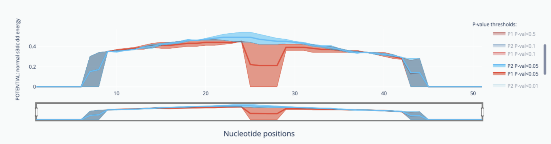
- By default, you will see a profile of the FIMO binding ratio. Switch this to POTENTIAL.
- The scoring profile will be displayed:
- The y-axis represents the structure-based potential score.
- The x-axis represents the nucleotide position.
- The SNP is always positioned in the middle.
- For further assistance interpreting results, refer to:
References
1) Abadi, M., Barham, P., Chen, J., Chen, Z., Davis, A., Dean, J., ... & Zheng, X. (2016). {TensorFlow}: a system for {Large-Scale} machine learning. In 12th USENIX symposium on operating systems design and implementation (OSDI 16) (pp. 265-283).
2) Abramov, S., Boytsov, A., Bykova, D., Penzar, D. D., Yevshin, I., Kolmykov, S. K., ... & Kulakovskiy, I. V. (2021). Landscape of allele-specific transcription factor binding in the human genome. Nature communications, 12(1), 2751.
3)Altschul, S. F., Gish, W., Miller, W., Myers, E. W., & Lipman, D. J. (1990). Basic local alignment search tool. Journal of molecular biology, 215(3), 403-410.
4) Bass, J. I. F., Sahni, N., Shrestha, S., Garcia-Gonzalez, A., Mori, A., Bhat, N., ... & Walhout, A. J. (2015). Human gene-centered transcription factor networks for enhancers and disease variants. Cell, 161(3), 661-673.
5) Chen J, Rozowsky J, Galeev TR, Harmanci A, Kitchen R, Bedford J, Abyzov A, Kong Y, Regan L, Gerstein M. A uniform survey of allele-specific binding and expression over 1000-Genomes-Project individuals (2016).
6) Coetzee, S. G., Coetzee, G. A., & Hazelett, D. J. (2015). motifbreakR: an R/Bioconductor package for predicting variant effects at transcription factor binding sites. Bioinformatics, 31(23), 3847-3849.
7) Gohl, P., Bonet, J., Fornes, O., Planas-Iglesias, J., Fernandez-Fuentes, N., & Oliva, B. (2023). SBILib: a handle for protein modeling and engineering. Bioinformatics, 39(10), btad613.
8) Grant, C. E., Bailey, T. L., & Noble, W. S. (2011). FIMO: scanning for occurrences of a given motif. Bioinformatics, 27(7), 1017-1018.
9) Gualdi, F., Oliva, B., & Pinero, J. (2024). Genopyc: a python library for investigating the genomic basis of complex diseases. bioRxiv, 2024-01.
10) Mistry, J., Chuguransky, S., Williams, L., Qureshi, M., Salazar, G. A., Sonnhammer, E. L., ... & Bateman, A. (2021). Pfam: The protein families database in 2021. Nucleic acids research, 49(D1), D412-D419.
11) Raney, B. J., Barber, G. P., Benet-Pagès, A., Casper, J., Clawson, H., Cline, M. S., ... & Haeussler, M. (2024). The UCSC Genome Browser database: 2024 update. Nucleic Acids Research, 52(D1), D1082-D1088.
12) Storey JD, Bass AJ, Dabney A, Robinson D (2023). qvalue: Q-value estimation for false discovery rate control. doi:10.18129/B9.bioc.qvalue, R package version 2.34.0, https://bioconductor.org/packages/qvalue.
13) Weirauch, M. T., Yang, A., Albu, M., Cote, A. G., Montenegro-Montero, A., Drewe, P., ... & Hughes, T. R. (2014). Determination and inference of eukaryotic transcription factor sequence specificity. Cell, 158(6), 1431-1443.
14) Zuo, C., Shin, S., & Keleş, S. (2015). atSNP: transcription factor binding affinity testing for regulatory SNP detection. Bioinformatics, 31(20), 3353-3355.